IQ2Spect
an I/Q to spectrogram forecasting machine learning model
Forecasting models in the radio domain play a huge role in spectrum resource management, where we must squeeze more performance out of finite spectrum for a rapidly growing device base. As of Q2 2025 there were about 2.6 billion 5G subscriptions worldwide, with two-thirds of all mobile subscriptions expected to be 5G by 2030—a shift that is also driving mobile data traffic up ~19% year-over-year to ~180 EB/month as of Q2 2025 [ericson-5g, ericson-net-traffic].
Meanwhile, the Internet of Things is exploding: cellular IoT connections approached ~4 billion at end-2024 and are forecast to exceed 7 billion by 2030, and broader IoT device counts are estimated at ~21 billion in 2025, on track for ~39 billion by 2030. Connected and automated vehicles (V2X) are part of this rise, with regulators actively preparing spectrum and policy frameworks to enable large-scale deployment [ericson-iot, iot-analytics,gsm-analytics].
With more users, devices, and data-hungry applications competing for airwaves, researchers increasingly turn to machine learning (ML) for tough radio-resource optimization problems (e.g., scheduling, power control, and dynamic spectrum access). Recent surveys and studies detail how ML-based approaches can predict spectral occupancy and guide real-time spectrum management [2025-survey, 2023-article].
In this work, we demonstrate that ML models can learn temporal patterns in wireless signals to forecast a future time window and we quantify how reliable these predictions are for practical spectrum-management decisions.
Consider a received complex baseband signal $r_t = I_t + jQ_t$ captured within a spectrum band of bandwidth $BW$. The band contains a mix of technologies—Wi-Fi, LTE, 5G, Bluetooth, etc.—producing overlapping, bursty traffic. Our question is simple: given a history of signals, can we predict a short window in the future? We set up a forecasting pipeline that ingests raw IQ from a software-defined radio (SDR), applies lightweight preprocessing, and feeds a ConvLSTM forecaster to predict a future spectrogram time slot, trained end-to-end with an MSE objective against ground truth spectrogram frames.

The system model shown above depicts the structure of our implementation. The received signal $r_t \in \mathbb{C}^k$ is the raw I/Q samples captured for $X$ms of length $k$. It is fed into the IQ2Spect pytorch model with two distinct blocks; the preprocessing block and the ConvLSTM network block. In order to accurately predict spectrograms we need to feed spectrograms, so the preprocessing block along with the transformation function $\mathcal{T}$ produces spectrogram frames of the history of I/Q samples that is fed to the ConvLSTM network. The ConvLSTM network then predicts a spectrogram map which in our experiments were three versions; FFT, masked and grided maps.
One observation is the length of the history window and the prediction, $X$ms and $Y$ms. First, we must ensure that the prediction is less than the history window i.e., $Y < X$ms. Also, in our implementation, we ensured that $X=f\times Y$ where $f$ is an integer factor. Suppose $X=16$ then $Y$ has to be an integer multiple of 16, say 2.
The preprocessing block
We decided to implement two versions of the preprocessing block. One where we train an FFT model which we termed learned and another were we implement and FFT operation in the forward pass which is indicated as not learned.
No special dataset is needed for this step due to the simplicity of the transformation function (the FFT matrix) to be learned. We thus used random values to learn the transformation by feeding a multi-layer perceptron (MLP) of N neurons (equivalent to N-point FFT operation) with concatenated the real and imaginary values. For details of the implementation check out repo fft-gist.
With all the variables in our system model, we ask the following questions to build our investigation on performance
- What is the performance of the model based on the FFT approach?
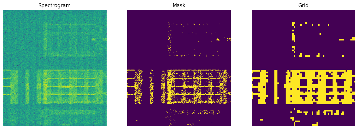
- What is the impact of different spectrogram map format (spectrogram, mask, or grid) on the performance of the model?
- What is the impact of different history time window ($X = $16ms or 20ms) on the performance of the model?
- What is the impact of different model sizes?
Results
We present the results on model performance with respect to the FFT approach, spectrogram format, length of history window, $X$ms and size of model while evaluating our model based on F1 score.
Let’s observe the performance of the model based on the FFT approach.
| Model | # of params (Million) | F1 score (%) | GPU inference time (ms) | CPU inference time (s) |
|---|---|---|---|---|
| IQ2Spect (learned FFT) | 13.68 | 30.63 | 52.59 | 15.9 |
| IQ2Spectv2 | 9.48 | 36.11 | 22.62 | 11.9 |
With FFT approach, the not learned method had the best performance, the least number of parameters, and quicker inference time on GPU and CPU. This is expected as the we eliminate the extra trainable parameters from the MLP layer which also has some margin of error compared to the actual FFT operation. Though we show that the FFT operation can be learned in the model. In the next set of results, we use the IQ2Spectv2 for further evaluation.
Let’s observe the impact of different spectrogram map formats (spectrogram, mask and grid)
| Model | # of params (Million) | F1 score |
|---|---|---|
| IQ2Spect | 9.48 | 36.11 |
| IQ2Mask | 9.48 | 28.69 |
| IQ2Grid | 0.64 | 49.71 |
In this investigation, the grid spectrogram map had the best performance compared to the others. This might be due to the simplicity of the prediction map compared to the others. For the spectrogram map, the loss objective is the MSE loss which computes the squared difference between the values of the prediction and the ground truth on a 256 by 256 grid. On the other hand, the masked spectrogram map also produces a 256 by 256 grid of values $\in \lbrace0,1\rbrace$ so that the loss function is a binary cross entropy evaluation. However we see that the granularity of the objective hurts performance compared to the vanilla spectrogram map. But when we downsample the masked spectrogram map to a grid of 64 by 64, which is a simpler perdiction map, we measure gains compared to the baseline. Additionally, the IQ2Grid model has fewer parameters and shows that the simple downsampling strategy leads to ~15x drop.
Let’s observe the impact of difference history length (16ms and 20ms) on the accuracy of the predictions
| History window ($X$ms) | F1 score (%) |
|---|---|
| 16 | 49.71 |
| 20 | 58.96 |
In the past results, we used ($X=16$) and ($Y=2$). While keeping our constraints ($X=f\times Y$) and ($Y<X$), we investigate two history window lengths, 16 and 20. Our findings show that a longer history window can improve performance; informally, increasing ($f$) gives the model more context and tends to raise prediction accuracy in our setup. This is largely inherent to how an LSTM works.
Why the LSTM benefits from longer history. An LSTM maintains a cell state ($c_t$) that acts like a running summary of the past, and it uses gates to decide what to remember, what to forget, and what to output:
\[\begin{aligned} i_t &= \sigma(W_i x_t + U_i h_{t-1} + b_i) && \text{(input gate)} \\ f_t &= \sigma(W_f x_t + U_f h_{t-1} + b_f) && \text{(forget gate)} \\ o_t &= \sigma(W_o x_t + U_o h_{t-1} + b_o) && \text{(output gate)} \\ \tilde{c}_t &= \tanh(W_c x_t + U_c h_{t-1} + b_c) && \text{(candidate state)} \\ c_t &= f_t \odot c_{t-1} + i_t \odot \tilde{c}_t \\ h_t &= o_t \odot \tanh(c_t) \end{aligned}\]With a longer ($X$), the LSTM sees more cycles, bursts, and idle gaps in the traffic mix (e.g., Wi-Fi duty cycles, LTE/NR scheduling periodicities). Its forget gate ($f_t$) can retain structure that persists across many steps while discarding short-lived noise. In other words, extra history isn’t just “more data”—it’s more chances for the gates to filter and aggregate the right evidence into ($c_t$), which stabilizes multi-step forecasts for ($Y$).
What this means for ($f=X/Y$). Raising ($f$) generally helps until diminishing returns: once the relevant temporal patterns are already captured (e.g., several scheduling periods), pushing (X) further mostly adds redundancy and potential noise. Practically, we see gains from ($X=16\rightarrow20$) because the effective memory of the LSTM (set by learned gate biases) can span that range; beyond that, benefits taper unless there are longer rhythms to exploit.
Trade-offs: longer (X) increases compute and can overfit slow drifts; keep dropout/weight decay, and prefer validation curves to pick (X). But within our constraint ($X=f\times Y$) with ($Y<X$), nudging ($f$) up gives the LSTM the temporal “runway” it needs to turn noisy frames into a cleaner, predictable future.
Let’s observe the impact of different model sizes
| Model size (MB) | F1 score (%) |
|---|---|
| 2.55 | 49.71 |
| 4.27 | 57.23 |
| 5.47 | 54.16 |
| 9.20 | 51.12 |
Lastly, we investigated the impact of model size. We vary two independent hyperparameters—num_layers (depth) and hidden_dim (width)—and evaluate a full 2×2 grid. This yields four models:
| Model size (MB) | num_layers | hidden_dim | model_name |
|---|---|---|---|
| 2.55 | 3 | 16 | iq2grid_x05 |
| 4.27 | 5 | 16 | iq2grid_x10 |
| 5.47 | 3 | 32 | iq2grid_x20 |
| 9.20 | 5 | 32 | iq2grid_x30 |
Because ConvLSTM parameters scale roughly like ($\mathcal{O}(L,H^2)$), width (hidden_dim) increases model size more aggressively than depth for the same kernel. We report sizes as parameters-only (FP32) to keep comparisons consistent. This evaluations were done for $X=16$ and $Y=2$. The best performing model is num_layer = 5 and hidden_dim = 16 and the result also shows that we gain performance more by increasing the depth than the width of the model.
One analysis missing in our investigation is the performance from combining the findings with the impact of history window length and model size. Technically, what would happen if we combine longer history window with deeper models, would the performance be maximized across both results or otherwise?
Now let’s shift gears to the strenghts and limitations of our model to quantify how reliable these predictions are for practical spectrum-management decisions. Here we offer a more subjective qualitative analysis and the numbers (quantitative analysis) might indicate differently.

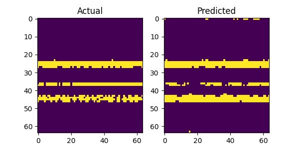
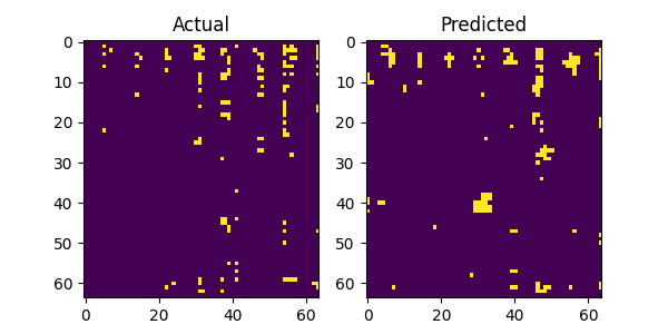

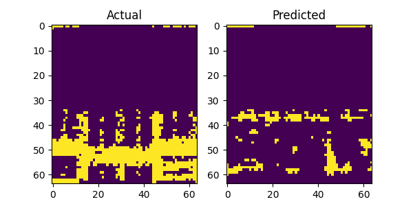

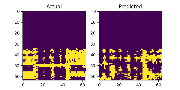
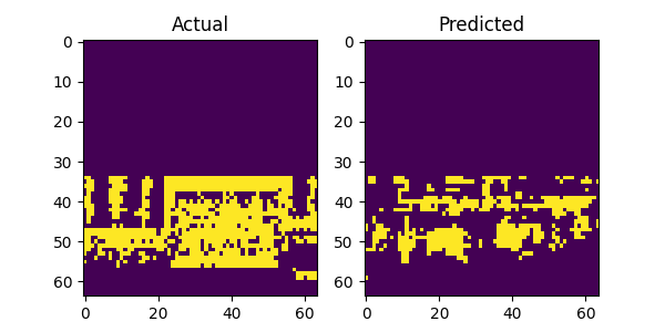
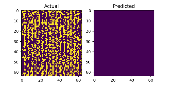
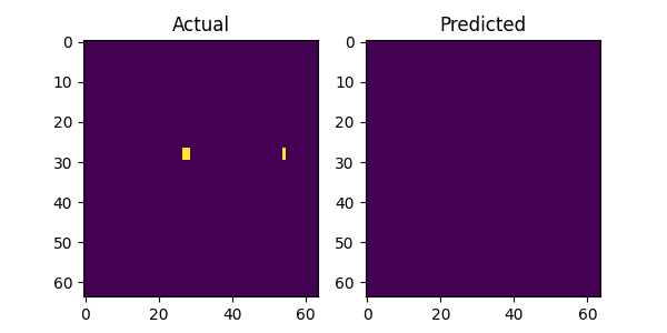
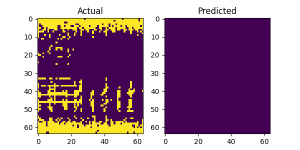
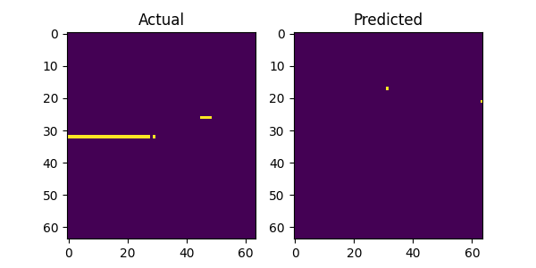
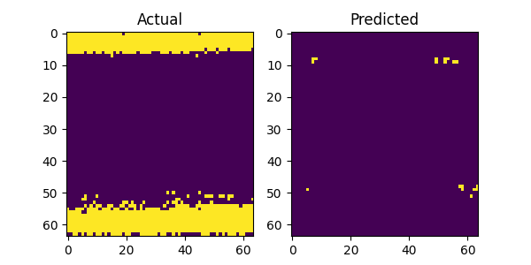
The above image gallery shows examples of impressive predictions from our system model. By mere observations, the model recognizes repeating patterns particularly for the LTE and 5G NR signals. This proves our initial intuition that machine learning models can recognize and learn temporal patterns in wireless technologies to make accurate forecast. However, when there is no recognizable pattern in the history window the model fails to produce accurate predictions as show in the following plots below. Additionally, there are examples where the model fails even when there is a recognizable pattern and we postulate that the bleeding signals in the receiver window as shown in the top and bottom areas of the figures attribute to the cause. It might confuse the model on what part to focus on when making predictions. This scenario with bleeding signals is also noticeable with the last figure where there are no periodic patterns and the model attempts to predict the bleeding signal.



Conclusion
IQ2Spect demonstrates that a compact, modular pipeline (raw I/Q → lightweight spectrogram transform → ConvLSTM forecaster) can reliably extract and exploit short-term temporal regularities in heterogeneous wireless traffic. Across our evaluations the model (a) learns repeatable LTE / NR scheduling rhythms, (b) benefits predictably from longer history windows (improved context without ballooning parameters), and (c) attains strong accuracy–efficiency balance: the not‑learned FFT path removes unnecessary trainable weights, the grid representation lifts F1 while shrinking parameter count ~15×, and deeper (rather than wider) ConvLSTM stacks yield better marginal gains. These strengths make the approach attractive for practical spectrum-management tasks such as proactive slot allocation, early detection of emerging contention, and low-latency dynamic spectrum access—where fast inference (≈22 ms GPU) and interpretable spectrogram outputs are key.
Current limitations are mostly side-effects of architectural inductive bias and the deliberate downsampling strategy: failures appear when temporal structure is weak or obscured by “bleeding” energy at band edges; coarse grids trade fine spectral detail for robustness and speed; and we have not yet jointly optimized longer histories with deeper stacks (potential compounding gains). These caveats do not undermine the core result—they highlight tunable knobs rather than fundamental barriers.
Overall, the system model is stronger at capturing and forecasting temporal patterns than the observed limitations might suggest. The consistent improvement from modest increases in history and careful representation choice indicates clear headroom for extension. Next steps focus on (1) broader testing and evaluation under dynamic radio conditions (varying traffic mixes, mobility, SNR, and interference regimes), and (2) investigating parallel processing with transformer‑based components while maintaining the LSTM lookback capability (e.g., hybrid LSTM–Transformer) to scale inference without sacrificing temporal context.
In short: IQ2Spect validates that temporal pattern learning from raw I/Q is both feasible and practically useful, with limitations attributable to choices we can iteratively refine—setting a solid foundation for next-generation spectrum forecasting models.